Introduction
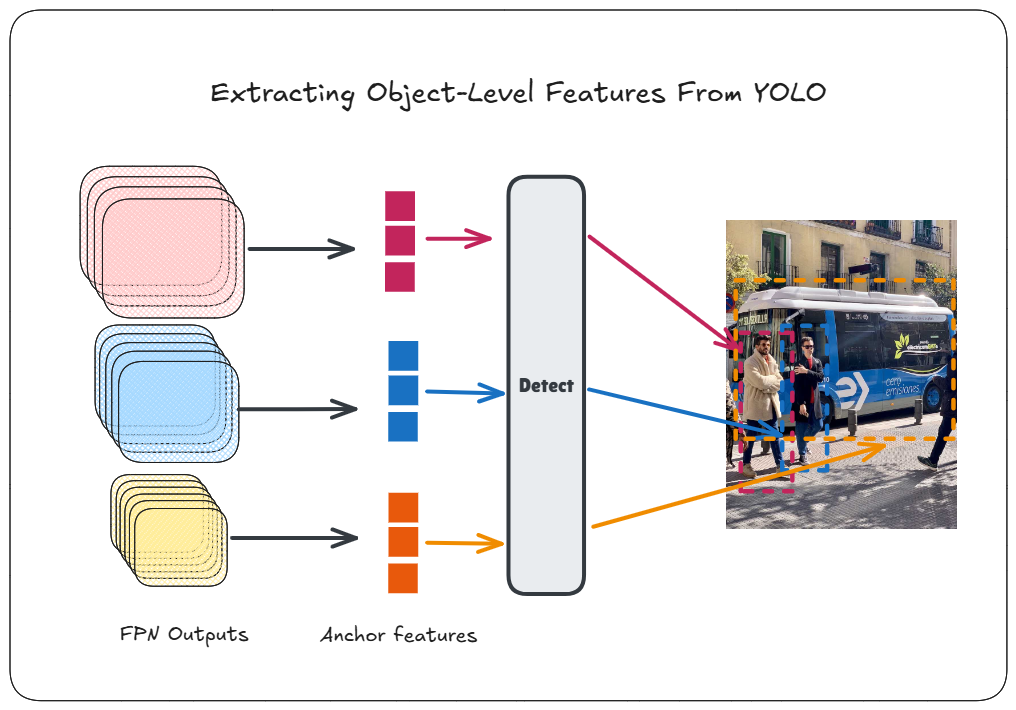
Every detected object in an object detection network has an associated feature used for the final prediction. These object-level features or embeddings from networks like YOLO are also valuable for various downstream tasks, such as similarity calculations used in re-identification. However, these features are not readily accessible, often leading people to use a separate network to obtain feature embeddings from object crops, which introduces unnecessary overhead.
In this guide, we will extract these features directly from ultralytics, thereby avoiding the additional overhead. The Colab notebook with all the steps can be found by clicking the “Open in Colab” badge above.
Modifications To Obtain The Features
ultralytics provides a way to retrieve the features of a particular layer through the embed argument. However, the features extracted through it are pooled and flattened. We will monkey-patch the _predict_once function so that it doesn’t do that and returns the features as they are:
# Update the method so that feature maps are returned without any modifications
def _predict_once(self, x, profile=False, visualize=False, embed=None):
    y, dt, embeddings = [], [], []  # outputs
    for m in self.model:
        if m.f != -1:
            x = y[m.f] if isinstance(m.f, int) else [x if j == -1 else y[j] for j in m.f]  # from earlier layers
        x = m(x)
        y.append(x if m.i in self.save else None)  # save output

        # Change this so that it returns the feature maps without any change
        if embed and m.i in embed:
            embeddings.append(x)  # flatten
            if m.i == max(embed):
                return embeddings
    return x

# Monkey patch method
model.model._predict_once = MethodType(_predict_once, model.model)
Next, we will initialize the predictor instance with the required arguments along with the layers from which we wish to extract the features:
# Initialize predictor so that we can perform preprocess, inference and postprocess ourselves.
_ = model("ultralytics/assets/bus.jpg", save=False, embed=[15, 18, 21, 22])
Here, we specify the layers 15, 18, 21 and 22. The first 3 layers are FPN outputs from the three FPN scales that are used by default in YOLOv8. You can find the layer numbers by checking model.model.yaml which shows the last layer using these as input:
[[15, 18, 21], 1, 'Detect', ['nc']]]
We also extract layer 22, since that’s the final layer with the actual predictions.
Running the previous code creates a predictor instance that can be used without having to call model.predict(). The benefit of this is that we can decouple the preprocessing, inference and postprocessing steps:
# Run inference
imgs = [cv2.imread("ultralytics/assets/bus.jpg")]
prepped = model.predictor.preprocess(imgs)
result = model.predictor.inference(prepped)
The result variable contains the outputs from layers 15, 18, 21, and 22 without any postprocessing applied. Before applying postprocessing, we need to modify the non_maximum_suppression() function to return the indices of the retained objects. This is necessary because the output from the last layer of YOLOv8n has the shape [1, 84, 8400]. This output is a concatenation of results from each FPN level: layer 15 produces 80x80 = 6400 anchors, layer 18 produces 40x40 = 1600 anchors, and layer 21 produces 20x20 = 400 anchors for an input of shape 640x640. The total number of anchors is 6400 + 1600 + 400 = 8400.
Each anchor has an associated feature used by the final layer to predict the location and class of objects. However, only a few anchors actually contain objects, which is why a confidence threshold and NMS are applied. To identify which anchors contributed to the final prediction, we need to modify the NMS function to return the indices of the 8400 outputs retained in the final postprocessed output. The modification is as follows:
 def non_max_suppression(
     prediction,
     conf_thres=0.25,
@@ -229,12 +230,19 @@ def non_max_suppression(
     mi = 4 + nc  # mask start index
     xc = prediction[:, 4:mi].amax(1) > conf_thres  # candidates

+    # To keep track of the prediction indices that remain at the end, we create an indices
+    # list that will be applied the same filters that get applied to the original predictions.
+    # That way, at the end, we will have xks with only the indices of the predictions that
+    # have not been eliminated.
+    xinds = torch.stack([torch.arange(len(i), device=prediction.device) for i in xc])[...,None]
     # Settings
     # min_wh = 2  # (pixels) minimum box width and height
     time_limit = 2.0 + max_time_img * bs  # seconds to quit after
@@ -243,10 +251,13 @@ def non_max_suppression(

     t = time.time()
     output = [torch.zeros((0, 6 + nm), device=prediction.device)] * bs
-    for xi, x in enumerate(prediction):  # image index, image inference
+    feati = [torch.zeros((0, 1), device=prediction.device)] * bs
+    for xi, (x, xk) in enumerate(zip(prediction, xinds)):  # image index, image inference
         # Apply constraints
         # x[((x[:, 2:4] < min_wh) | (x[:, 2:4] > max_wh)).any(1), 4] = 0  # width-height
-        x = x[xc[xi]]  # confidence
+        filt = xc[xi]
+        x = x[filt]  # confidence
+        xk = xk[filt] # indices update

         # Cat apriori labels if autolabelling
         if labels and len(labels[xi]) and not rotated:
@@ -266,20 +277,27 @@ def non_max_suppression(
         if multi_label:
             i, j = torch.where(cls > conf_thres)
             x = torch.cat((box[i], x[i, 4 + j, None], j[:, None].float(), mask[i]), 1)
+            xk = xk[i] # indices update
         else:  # best class only
             conf, j = cls.max(1, keepdim=True)
-            x = torch.cat((box, conf, j.float(), mask), 1)[conf.view(-1) > conf_thres]
+            filt = conf.view(-1) > conf_thres
+            x = torch.cat((box, conf, j.float(), mask), 1)[filt]
+            xk = xk[filt] # indices update

         # Filter by class
         if classes is not None:
-            x = x[(x[:, 5:6] == classes).any(1)]
+            filt = (x[:, 5:6] == classes).any(1)
+            x = x[filt]
+            xk = xk[filt] # indices update

         # Check shape
         n = x.shape[0]  # number of boxes
         if not n:  # no boxes
             continue
         if n > max_nms:  # excess boxes
-            x = x[x[:, 4].argsort(descending=True)[:max_nms]]  # sort by confidence and remove excess boxes
+            filt = x[:, 4].argsort(descending=True)[:max_nms]
+            x = x[filt]  # sort by confidence and remove excess boxes
+            xk = xk[filt] # indices update

         # Batched NMS
         c = x[:, 5:6] * (0 if agnostic else max_wh)  # classes
@@ -305,11 +323,15 @@ def non_max_suppression(
         #         i = i[iou.sum(1) > 1]  # require redundancy

         output[xi] = x[i]
+        # xk would contain the indices of the predictions that are in x,
+        # i.e. you could index the `prediction` variable at the beginning of this function
+        # and get the final x (in xyxy format)
+        feati[xi] = xk[i].reshape(-1)
         if (time.time() - t) > time_limit:
             LOGGER.warning(f"WARNING ⚠️ NMS time limit {time_limit:.3f}s exceeded")
             break  # time limit exceeded

-    return output
+    return output, feati
We then use it to process the output of the final layer (layer 22; result[-1]):
# This would return the NMS output in xywh format and the idxs of the predictions that were retained.
output, idxs = non_max_suppression(result[-1][0], in_place=False)
Once we have indices of the anchors that were retained, we can then use it to get the feature vector by indexing into the grid cell of the FPN output corresponding to a particular anchor:
def get_object_features(feat_list, idxs):
    # feat_list would contain feature maps in grid format (N, C, H, W), where each (H,W) is an anchor location.
    # We permute and then flatten the grid so that each grid and its feature vectors
    # correspond with the indexes of the prediction. We also downsample the vector to the smallest one (64).
    obj_feats = torch.cat([x.permute(0, 2, 3, 1).reshape(x.shape[0], -1, 64, x.shape[1] // 64).mean(dim=-1) for x in feat_list], dim=1)
    return [feats[idx] for feats, idx in zip(obj_feats, idxs)] # for each image in batch, indexed separately

# Get features of every detected objected in the final output for every image in batch.
obj_feats = get_object_features(result[:3], idxs)
We pass the outputs from layers 15, 18, and 21 to get_object_features(), along with the indices of the final objects. However, these outputs do not have the same number of channels or feature vector lengths. To compare features from different FPN levels, we downsample the longer feature vectors to the shortest length, which is 64, using mean reduction.
Next, we concatenate the flattened grids in the same order as the final layer concatenated the outputs from these layers. This ensures that the order of anchors matches the order of the 8400 outputs we saw earlier, allowing us to use the indices obtained from NMS to retrieve the corresponding feature vectors.
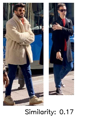
The obj_feats variable will contain the feature vectors in the order of the boxes in the results. Therefore, if you want to compare the feature vector of the first box with the second box, you can simply run:
# Similarity between first and second object
# The order corresponds to the order of boxes in results below
>>> i = 0  # first image in batch
>>> cosine_similarity(obj_feats[i][0], obj_feats[i][1], dim=0)
tensor(0.3843, device='cuda:0')
We can combine this in a single function so that you get both the features along with the usual ultraytics Results object:
# Combined function
def get_result_with_features(imgs):
  # Run inference
  imgs = [cv2.imread(img) for img in imgs]
  prepped = model.predictor.preprocess(imgs)
  result = model.predictor.inference(prepped)

  # This would return the NMS output in xywh format and the idxs of the predictions that were retained.
  outputs, idxs = non_max_suppression(result[-1][0], in_place=False)

  # Get features of every detected objected in the final output.
  obj_feats = get_object_features(result[:3], idxs)

  # Also turn the original inference output into results
  results = []
  for img, output, feat in zip(imgs, outputs, obj_feats):
      output[:, :4] = scale_boxes(prepped.shape[2:], output[:, :4], img.shape)
      result = Results(img, path="", names=model.predictor.model.names, boxes=output)
      result.feats = feat
      results.append(result)

  return results

results_with_feat = get_result_with_features([ASSETS / "bus.jpg"])

# You can now easily access the box along with the features of that particular box
result = results_with_feat[0]
for box, feat in zip(result.boxes.xyxy, result.feats):
  # Use box or feat

Comparison with ResNet50
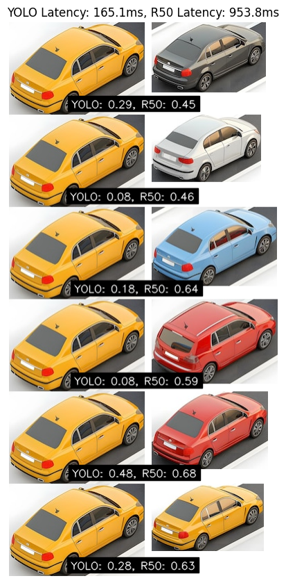
Let’s compare the similarity scores and latency between ResNet50 features and the object-level features extracted from YOLO.

At the bottom of each pair, are the cosine similarity scores calculated based on YOLO and ResNet50 embeddings.
ResNet50 is noticeably slower, taking 953.8ms to extract embeddings from all individual object crops, whereas YOLO completes detection and feature extraction in 165.1ms. These latencies were measured on Google Colab’s CPU instance. The latency of ResNet50 would also increase with increase in number of instances.
In terms of similarity scores, ResNet50 embeddings provides relatively higher scores, even for visually dissimilar pairs such as the second and the fourth pairs. The embeddings from YOLO, on the other hand, provide lower similarity scores in general, but they also discriminate better between similar and dissimilar pairs. For example, the least similar pairs based on the YOLO embeddings are the second and fourth pairs, which are indeed different vehicles. In contrast, the ResNet50 embeddings produce the lowest score for the first pair, which actually are similar vehicles differing mainly in color.
Conclusion
This guide explored how to extract object-level features directly from YOLO using ultralytics. Unlike traditional approaches that require cropping detected objects and running a separate embedding network on each crop, this method avoids that extra overhead. It enables feature-based similarity calculations to be integrated into downstream tasks with minimal latency. We also compared YOLO’s object embeddings to ResNet50. While YOLO’s embeddings produced lower similarity scores, they were however more disciminative and significantly faster to obtain.
Thanks for reading.