A Simple Trick To Increase YOLOv8's Accuracy On Small Objects With No Overhead

Introduction

Small object detection is usually a challenging task since the size of the objects makes it difficult for the features to be adequately represented in the backbone. There have been numerous improvements in object detection architectures over the years to increase small object detection accuracy. Such as the addition of feature pyramid layers that produce feature maps at multiple scales to ensure the extracted features have both coarse and fine features. YOLOv8 provides two additional variants that make use of extra scales to help with small and large object detection, namely the p2 and p6 models respectively. However, the p2 model comes with an additional cost due to the extra feature scale that gets added. For example, the original YOLOv8n model consumes 8.9 GFLOPs while the YOLOv8n-p2 model almost doubles that to 17.4 GFLOPs:

YOLOv8n-p2 summary: 277 layers, 3354144 parameters, 3354128 gradients, 17.4 GFLOPs
(277, 3354144, 3354128, 17.4345728)

Besides the difficulty in representing the features of small objects, there’s another reason why you might observe low mAP in small object detection, which is the use of IoU-based loss. For small objects, IoU is not a good metric to measure performance because small discrepancies in the predictions can often lead to large variations in loss, making the training less stable. You can read this article by Deci AI for a more detailed explanation on why that’s the case. It also discusses why mAP50-95 isn’t appropriate for measuring the performance of a detector on small objects.

A better target while training an object detector to detect small objects is the distance between the centers of the predicted and ground-truth boxes. This makes the loss less sensitive to the predicted box not accurately “hugging” the object, which is not a big deal for small objects as the difference is visually negligible. There is a simple trick that can be used to do this with YOLOv8, which I will explain in the next few sections. The whole code can be found in this Colab notebook.

An Example: TT100K Dataset

TT100K dataset is a large-scale dataset for traffic sign detection and classification made available by the Tencent Lab at Tsinghua University. Since it involves detecting traffic signs, it naturally consists of a lot of small objects. This makes it suitable for testing our theory. I won’t be using the whole dataset here (since I don’t have a GPU to run it for that long), and instead, I will be using the one from Roboflow that has about 20k images. We will first train a normal YOLOv8n model to test our mileage. I only ran it for just 10 epochs because Colab’s generosity ends too quickly for me to do anything more:

results = model.train(data="/content/Traffic-Signs-8/data.yaml", batch=-1, epochs=10,
                      warmup_epochs=1, close_mosaic=1, hsv_h=0, hsv_v=0, hsv_s=0,
                      scale=0, shear=0, translate=0)

I disabled augmentations as the Roboflow dataset is pre-augmented and since it also speeds up the training. I reduced the warmup_epochs and close_mosaic to 1 as we are running it for just 10 epochs. Here are the results after the 10 epochs:

Model summary (fused): 168 layers, 3015008 parameters, 0 gradients, 8.1 GFLOPs
                 Class     Images  Instances      Box(P          R      mAP50  mAP50-95): 100%|██████████| 25/25 [00:35<00:00,  1.42s/it]
                   all       2017       4906      0.467      0.461      0.448      0.326

We reached an mAP50 of 44.8, which is not bad considering it’s the nano version and was only trained for 10 epochs. But let’s see how much better we can do with our trick.

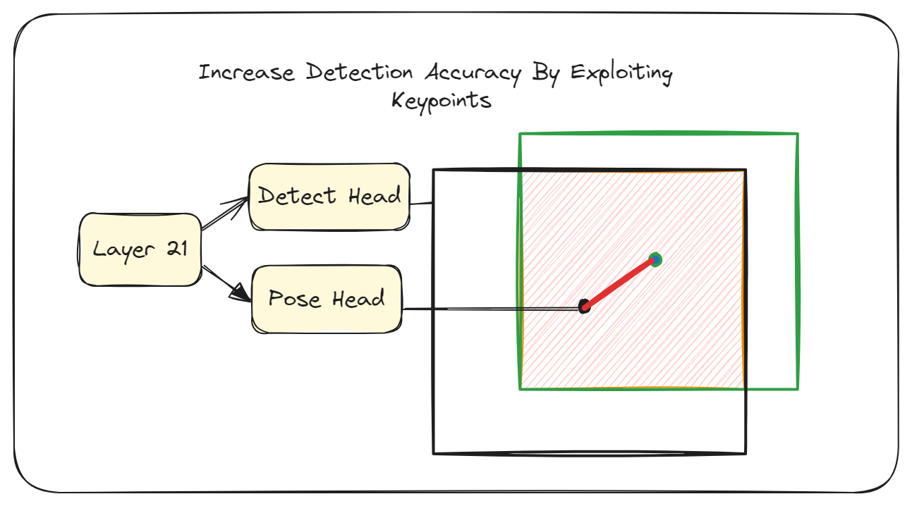
Keypoints To The Rescue

You may be familiar with the pose family of YOLOv8 models that can be used to perform keypoint estimation. The YOLOv8 pose models under the hood are just the detection models but with an additional pose head added to make keypoint prediction possible. This information will come in handy later, but right now, we want to exploit the keypoints to do what was mentioned in the introduction, i.e. train the model using the distance to the center as a target as opposed to IoU. To do this, we first convert our box labels to keypoint labels with this simple script:

labels = glob("/content/Traffic-Signs-8/*/labels/*.txt", recursive=True)

root_dir = Path(labels[0]).parent.parent.parent
for label in labels:
    label = Path(label)
    split = label.parent.parent.name
    img_path = [(root_dir / split / "images" / label.with_suffix(sfx).name)
                for sfx in [".png", ".jpg", ".PNG", ".JPG"]]
    img_path = [pth for pth in img_path if pth.exists()][0]
    boxes = []
    points = []
    classes = []
    save_pth = root_dir / split / "labels_kp" / label.name
    save_pth.parent.mkdir(exist_ok=True)
    with open(label) as f:
        lines = f.readlines()
        for line in lines:
            splits = line.rstrip().split(" ")
            cls_id = int(splits[0])
            box = splits[1:]
            if not box:
                with open(save_pth, "w") as f:
                    pass
                continue

            box = [float(pt) for pt in box]
            point = (box[0], box[1])
            points.append(point)
            boxes.append(box)
            classes.append(cls_id)

    with open(save_pth, "w") as f:
        for point, box, cls_id in zip(points, boxes, classes):
            f.writelines(f"{cls_id} {box[0]} {box[1]} {box[2]} {box[3]} {point[0]} {point[1]} 1 \n")

The code is pretty self-explanatory, but the gist of it is that we use the x and y coordinates of the boxes, representing the center, as the keypoint and also set the keypoint visibility to 1. So the format used is class_id x y w h kp_x kp_y visibility. Then we append the kpt_shape to the existing data.yaml file which is required for the training to work:

# Add keypoint shape to data.yaml
echo "kpt_shape: [1, 3]" >> /content/Traffic-Signs-8/data.yaml

Now, we just start training:

results = model.train(data="/content/Traffic-Signs-8/data.yaml", batch=41, epochs=10,
                      box=0.01, dfl=0.01, warmup_epochs=1, close_mosaic=1, hsv_h=0,
                      hsv_v=0, hsv_s=0, scale=0, shear=0, translate=0)

Most of the configuration here is the same as the previous training. The batch size is explicitly specified since the auto mode in the previous training selected 41, and we want to use the same batch size to ensure the comparison is fair. The only difference is that the box and dfl loss weights are reduced to 0.01. This means that the loss would largely be influenced by the keypoints rather than the boxes, making the training less sensitive to discrepancies in IoU. With these settings, I got the following results after 10 epochs:

YOLOv8n-pose summary (fused): 187 layers, 3086681 parameters, 0 gradients, 8.4 GFLOPs
                 Class     Images  Instances      Box(P          R      mAP50  mAP50-95)     Pose(P          R      mAP50  mAP50-95): 100%|██████████| 25/25 [00:38<00:00,  1.54s/it]
                   all       2017       4906      0.581      0.476      0.506      0.319       0.57      0.508      0.541      0.537

Despite reducing the box and dfl loss weights, we get over a 12% increase in the box mAP50 from using the keypoint targets, going from 44.8 in the previous training to 50.6 using the pose-based model. However, we see a slightly lower map50-95 score. This is because, as was mentioned, small object detection is very sensitive to IoU changes and since mAP50-95 averages the performance at higher IoU thresholds, it scores lower. However, in reality, the model performs better than the normal detection model in small object detection. There’s also pose mAP in the results above which you can ignore since it’s for the pseudo-keypoints we created.

Bringing Out The Detect In Pose

If you look at the results shown in the previous section, you will notice that the pose model shows 8.4 GFLOPs while the detect model had shown 8.1 GLOPs. These extra FLOPs come from the pose head. But don’t worry. We can get it back down to 8.1 GFLOPs. Remember that I mentioned YOLOv8 pose models are just detection models with a pose head attached? Well, this also means that we can turn our pose model back to a detect model without losing any accuracy at all while removing the extra overhead introduced by the pose head.

First, we edit the yaml to match the number of classes in the pose model so that the last layer weights don’t have an issue loading:

# Change nc to correct number of classes
sed -i "s/nc:.*$/nc: 48/g" ultralytics/cfg/models/v8/yolov8.yaml

Then we just need these few lines to turn the pose model into a detection only variant:

# Converting pose to detect
model_d = YOLO("ultralytics/cfg/models/v8/yolov8n.yaml").load(model.model)
model_d.ckpt = {"model": model_d.model}
model_d.save("best_detect.pt")

Here, we load the weights of the pose model to a detect model, and they match up perfectly since all the layers until the pose head are identical, and we save that new model as best_detect.pt.

To verify that no performance was lost, we can just run validation again. And it gives the following output:

YOLOv8n summary (fused): 168 layers, 3015008 parameters, 21840 gradients, 8.1 GFLOPs
                 Class     Images  Instances      Box(P          R      mAP50  mAP50-95): 100%|██████████| 127/127 [00:31<00:00,  4.08it/s]
                   all       2017       4906      0.586      0.474      0.507       0.32

You can see that all the metrics are pretty much the same, in fact, it’s a bit higher here and the FLOPs count shows 8.1 which is what we had with the original detect model.

Conclusion

The training here was only run for 10 epochs, but you should be able to observe the differences becoming significant as you train for longer. It may be helpful even if you aren’t particularly targeting small objects as the pose head provides an auxiliary task during training and auxiliary tasks have been shown to help the model learn better. You can turn segmentation models into detect by using the same approach as in the last section which is another auxiliary task you can try to improve your model’s detection performance.

Thanks for reading.